 Q3 2026Quarterly report
Entries gained share while instruction activity fell
Instruction activity and composition across Q3, with complete May and June observations, labelled available-period Q2 comparisons, conditional Q4 activity cases and a separate external macro assessment.
On this page
1. Abstract
This report examines Q3 instruction activity, composition and timing, with complete May and June observations and matched available-Q2/Q3 windows. In the matched-period comparison, the standardised entry rate fell 11.1% while entry share rose from 52.9% to 61.8%. Gold’s share recovered within Q3 but remained below June’s; crypto grew against the available Q2 window while losing share within Q3. Calendar correction and within-class decomposition show why a single total cannot describe these movements. Eighteen numbered figures separate historical instruction observations, conditional Q4 sensitivity exercises and a distinct external macro outlook. The outlook applies explicit weekday-rate and composition assumptions to October, November, December and the quarter. It assigns no probabilities, estimates no confidence bands and incorporates no October instruction observations. The external outlook uses public releases checked on 11 October with their separate source dates. Results concern received instructions and recognised fields, with an unconfirmed source clock.
2. Data and comparison design
The observed unit is the recognised instruction received by the bridge, under the aligned source-instruction rule. Complete Q3 covers 1 July–30 September. The available-period comparison covers 10 April–30 June versus 10 July–30 September; it is not a complete-Q2 comparison. available April, May, June and September were read for this research on 11 October, while July and August use approved release handoffs. The source vintages are explicit and the eligibility definitions are aligned.
A standardised week sums the average Monday, Tuesday, Wednesday, Thursday, Friday, Saturday and Sunday in each window. Quarter shares are weighted from the underlying quarter aggregates. Activity changes and decomposition values are calculated before presentation rounding. No platform levels or participant-denominator measures are disclosed. A larger share need not accompany more activity, and recognised exit fields do not establish broker-side protection. Sources and scope notes accompany each figure; the CSV figure data accompanies this report.
The longer record changes the quarter’s interpretation. In matched available-period windows, entry instructions took a larger share even though entry activity fell. Management and other instructions fell more sharply. Within Q3, Gold gained share in each month, but September remained below June’s Gold share. Crypto lost share inside Q3 while its activity grew against the available Q2 window.
The comparison is deliberately bounded: 10 April–30 June against 10 July–30 September, using the source calendar. The source does not retain 1–9 April, so no full-Q2 pooled statistic is presented. Complete May and June observations are also shown beside the Q3 months. The matched windows contain different mixes of weekdays, so raw activity changes and standardised-week changes are reported separately. The standardised week adds each window’s average Monday, Tuesday and so on through Sunday.
Pulse measures recognised historical instructions received by the bridge, counted at their source. Instruction receipt does not establish what happened at a broker. The source timezone remains unconfirmed; these are source-calendar comparisons, not precise alignments with Singapore time or market announcements.
3. The whole quarter and its monthly path answer different questions
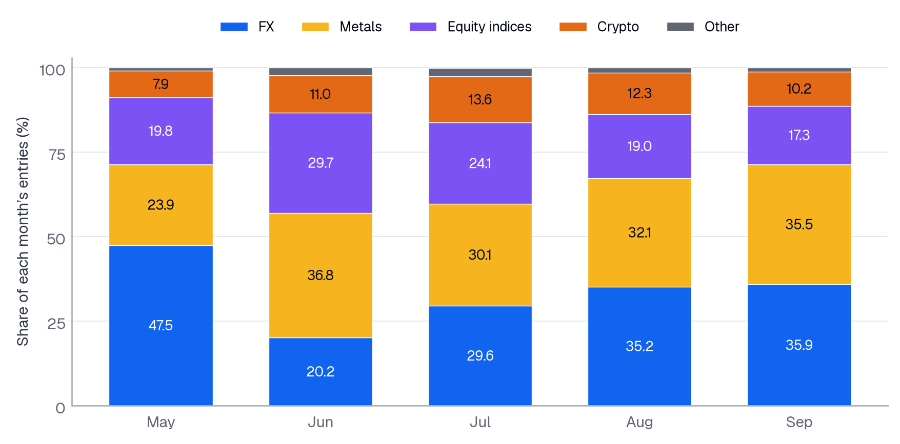
Complete source-calendar months. Shares are independently rounded; stacked totals may differ slightly from 100%. July/August use their approved earlier handoffs.
Source: PineConnector Pulse; received instruction aggregates. Shares are instruction-weighted. Download data (CSV): Figure 1
View figure data
| Series | Period | Value | Unit / kind |
|---|---|---|---|
| FX | 2026-05 | 47.5 | share of entry instructions %; observed |
| FX | 2026-06 | 20.2 | share of entry instructions %; observed |
| FX | 2026-07 | 29.6 | share of entry instructions %; observed |
| FX | 2026-08 | 35.2 | share of entry instructions %; observed |
| FX | 2026-09 | 35.9 | share of entry instructions %; observed |
| Metals | 2026-05 | 23.9 | share of entry instructions %; observed |
| Metals | 2026-06 | 36.8 | share of entry instructions %; observed |
| Metals | 2026-07 | 30.1 | share of entry instructions %; observed |
| Metals | 2026-08 | 32.1 | share of entry instructions %; observed |
| Metals | 2026-09 | 35.5 | share of entry instructions %; observed |
| Equity indices | 2026-05 | 19.8 | share of entry instructions %; observed |
| Equity indices | 2026-06 | 29.7 | share of entry instructions %; observed |
| Equity indices | 2026-07 | 24.1 | share of entry instructions %; observed |
| Equity indices | 2026-08 | 19.0 | share of entry instructions %; observed |
| Equity indices | 2026-09 | 17.3 | share of entry instructions %; observed |
| Crypto | 2026-05 | 7.9 | share of entry instructions %; observed |
| Crypto | 2026-06 | 11.0 | share of entry instructions %; observed |
| Crypto | 2026-07 | 13.6 | share of entry instructions %; observed |
| Crypto | 2026-08 | 12.3 | share of entry instructions %; observed |
| Crypto | 2026-09 | 10.2 | share of entry instructions %; observed |
| Other | 2026-05 | 0.9 | share of entry instructions %; observed |
| Other | 2026-06 | 2.3 | share of entry instructions %; observed |
| Other | 2026-07 | 2.5 | share of entry instructions %; observed |
| Other | 2026-08 | 1.4 | share of entry instructions %; observed |
| Other | 2026-09 | 1.1 | share of entry instructions %; observed |
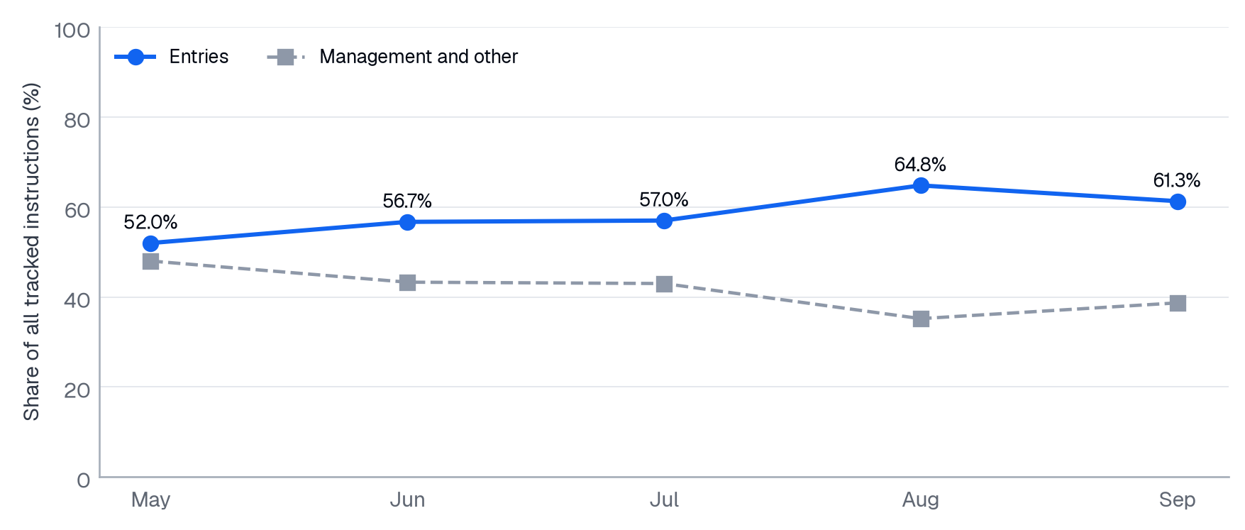
Management-and-other share is the complement of entry share. Composition is distinct from the level of activity.
Source: PineConnector Pulse; received instruction aggregates. Shares are instruction-weighted. Download data (CSV): Figure 2
View figure data
| Series | Period | Value | Unit / kind |
|---|---|---|---|
| Entries | 2026-05 | 52.0 | share of all tracked instructions %; observed |
| Entries | 2026-06 | 56.7 | share of all tracked instructions %; observed |
| Entries | 2026-07 | 57.0 | share of all tracked instructions %; observed |
| Entries | 2026-08 | 64.8 | share of all tracked instructions %; observed |
| Entries | 2026-09 | 61.3 | share of all tracked instructions %; observed |
| Management and other | 2026-05 | 48.0 | share of all tracked instructions %; observed |
| Management and other | 2026-06 | 43.3 | share of all tracked instructions %; observed |
| Management and other | 2026-07 | 43.0 | share of all tracked instructions %; observed |
| Management and other | 2026-08 | 35.2 | share of all tracked instructions %; observed |
| Management and other | 2026-09 | 38.7 | share of all tracked instructions %; observed |
Across the complete July–September quarter, entries represented 61.0% of all tracked instructions. FX and metals together supplied 66.3% of entries, including Gold at 32.3%. These quarter-wide shares are calculated from the underlying quarter aggregates. They are not an average of monthly percentages.
| Share of Q3 entry instructions | Whole-quarter share |
|---|---|
| Foreign exchange | 33.7% |
| Metals | 32.6% |
| Equity indices | 20.1% |
| Crypto | 12.0% |
| Other / unclassified | 1.7% |
Gold is a subset of metals, not another class. The following monthly table shows how the mix reached its quarter-wide result. Its denominator is each month’s own instruction stream, so its columns should not be pooled by averaging.
| Measure | May | June | July | August | September |
|---|---|---|---|---|---|
| Entries: share of all tracked instructions | 52.0% | 56.7% | 57.0% | 64.8% | 61.3% |
| FX: share of entries | 47.5% | 20.2% | 29.6% | 35.2% | 35.9% |
| Metals: share of entries | 23.9% | 36.8% | 30.1% | 32.1% | 35.5% |
| FX + metals: share of entries | 71.4% | 57.0% | 59.7% | 67.3% | 71.4% |
| Gold: share of entries | 23.4% | 36.4% | 29.7% | 31.8% | 35.2% |
| Equity indices: share of entries | 19.8% | 29.7% | 24.1% | 19.0% | 17.3% |
| Crypto: share of entries | 7.9% | 11.0% | 13.6% | 12.3% | 10.2% |
| Neither recognised exit field: share of entries | 58.9% | 41.0% | 32.8% | 29.1% | 31.8% |
| Average weekend day / average weekday entry rate | 12.3% | 14.7% | 14.9% | 13.4% | 11.3% |
Source vintages are explicit: the available April data and complete May, June and September were read on 11 October; July and August use the approved release handoffs. Their definitions are aligned across those vintages. May and June are complete source-calendar months. July–September match the aligned monthly observations in the released September edition; the original July growth headline is not joined to this sequence because its earlier eligibility treatment differs. Released September observations.
4. July, August and September told different stories
July established the quarter’s starting mix
The aligned July observation was the broadest of the three months by asset-class composition. FX and metals represented 59.7% of entries, with indices and crypto retaining larger shares than in the later months. Gold already led the named-market record at 29.7%. Entry commands made up 57.0% of all tracked instructions; the average weekend day carried 14.9% of an average weekday’s entry activity.
These levels establish the starting point for the Q3 comparison. They do not establish July’s change from Q2. The original July report compared with June under an earlier eligibility treatment, so its growth headline is not joined to this aligned sequence as though all figures shared one source definition.
August strengthened the rotation while the calendar hid activity
August’s clearest distinction was between entry growth and the total instruction headline. Entries increased while management and other instructions contracted. FX and metals reached 67.3% of entries, Gold rose to 31.8%, and entries reached 64.8% of the tracked stream. The average weekend-day rate eased to 13.4% of a weekday.
A lower raw total could therefore coexist with a busier standardised week and a more entry-heavy instruction mix. August did not simply become quieter. The calendar, class mix and command mix moved in different directions.
September preserved the rotation but weakened at the close
By September, FX and metals reached 71.4% of entries and Gold 35.2%. Entry share retraced to 61.3% as management activity increased. The average weekend-day rate eased further to 11.3% of a weekday.
The monthly composition extended August’s rotation, but the activity timeline broke from it: the early September window was above August’s standardised entry baseline, while the closing window was below it. A stable monthly entry total was therefore a poor description of the month’s path. The detailed split below separates those two observations without assigning them an unverified cause.
5. Entries gained share in the smaller matched-period stream
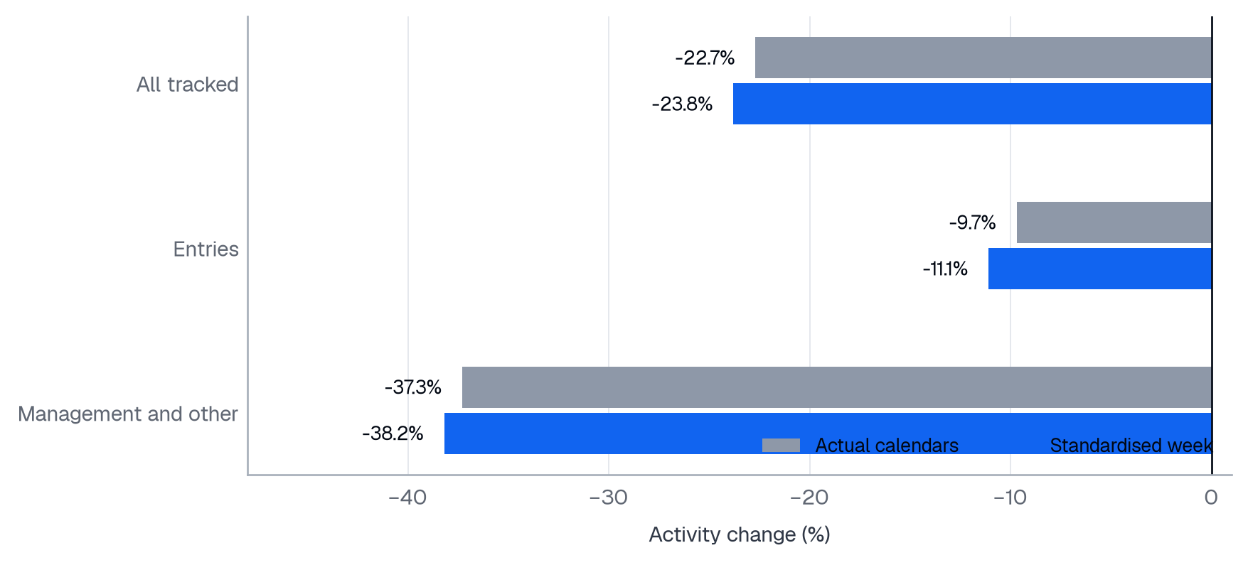
Available-period comparison, not full Q2. Standardisation sums the average of each weekday type.
Source: PineConnector Pulse; received instruction aggregates. Shares are instruction-weighted. Download data (CSV): Figure 3
View figure data
| Series | Period | Value | Unit / kind |
|---|---|---|---|
| All tracked / Actual calendars | 10 Jul–30 Sep versus 10 Apr–30 Jun | -22.7 | activity change %; observed |
| Entries / Actual calendars | 10 Jul–30 Sep versus 10 Apr–30 Jun | -9.7 | activity change %; observed |
| Management and other / Actual calendars | 10 Jul–30 Sep versus 10 Apr–30 Jun | -37.3 | activity change %; observed |
| All tracked / Standardised week | 10 Jul–30 Sep versus 10 Apr–30 Jun | -23.8 | activity change %; observed |
| Entries / Standardised week | 10 Jul–30 Sep versus 10 Apr–30 Jun | -11.1 | activity change %; observed |
| Management and other / Standardised week | 10 Jul–30 Sep versus 10 Apr–30 Jun | -38.2 | activity change %; observed |
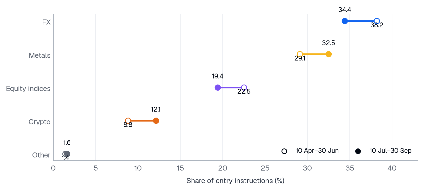
Open markers are the available Q2 window; filled markers are the matched Q3 window. No missing April dates were filled.
Source: PineConnector Pulse; received instruction aggregates. Shares are instruction-weighted. Download data (CSV): Figure 4
View figure data
| Series | Period | Value | Unit / kind |
|---|---|---|---|
| FX | 10 Apr–30 Jun | 38.2 | share of entry instructions %; observed |
| FX | 10 Jul–30 Sep | 34.4 | share of entry instructions %; observed |
| Metals | 10 Apr–30 Jun | 29.1 | share of entry instructions %; observed |
| Metals | 10 Jul–30 Sep | 32.5 | share of entry instructions %; observed |
| Equity indices | 10 Apr–30 Jun | 22.5 | share of entry instructions %; observed |
| Equity indices | 10 Jul–30 Sep | 19.4 | share of entry instructions %; observed |
| Crypto | 10 Apr–30 Jun | 8.8 | share of entry instructions %; observed |
| Crypto | 10 Jul–30 Sep | 12.1 | share of entry instructions %; observed |
| Other | 10 Apr–30 Jun | 1.4 | share of entry instructions %; observed |
| Other | 10 Jul–30 Sep | 1.6 | share of entry instructions %; observed |
The windows below are matched by the date from which the source remains available: 10 April–30 June and 10 July–30 September. They are not complete-quarter totals. The later window has one additional calendar day, and its weekday mix differs. A standardised week compares the average of each weekday type in each window; it does not remove changes in strategy composition or identify their causes.
| Instruction activity | Raw change between available windows | Standardised-week change |
|---|---|---|
| All tracked instructions | -22.7% | -23.8% |
| Entry instructions | -9.7% | -11.1% |
| Management and other instructions | -37.3% | -38.2% |
The standardised entry rate fell 11.1%, while management and other instructions fell 38.2%. Entry share nevertheless rose from 52.9% to 61.8%. A larger entry share therefore describes the relative contraction of the two instruction groups, not entry growth.
| Composition of entry instructions | 10 Apr–30 Jun | 10 Jul–30 Sep |
|---|---|---|
| Foreign exchange | 38.2% | 34.4% |
| Metals | 29.1% | 32.5% |
| Equity indices | 22.5% | 19.4% |
| Crypto | 8.8% | 12.1% |
| Other / unclassified | 1.4% | 1.6% |
FX and metals together took 67.3% and 66.9% of the respective streams, a much smaller difference than their rising monthly share inside Q3 suggests. Their internal balance changed: FX lost weight and metals gained it. Gold’s share rose from 28.6% to 32.2%.
Crypto supplies the counterexample to a simple ‘Q3 moved away from crypto’ story. Its share declined across the Q3 months, but its entry activity in the later matched window was 23.7% above the available Q2 window, or 22.7% above on a standardised week. A within-quarter decline and a positive comparison with an earlier window can both be true. The baseline determines which question the number answers.
The strongest limit is the missing early-April record. It could change a complete-quarter result, so these observations should not be renamed a full Q2-to-Q3 comparison. The matched-window approach keeps the observed periods explicit. It does not reconstruct the missing dates or prove that the available period represents the omitted one.
June changed the starting point for Q3
The standardised entry rate fell 48.4% from May to June, then rose 13.0% from June to July. June’s FX entry activity fell 77.0% on calendar months, while its Gold entry activity fell 16.0%. Because FX fell much more sharply, Gold’s share rose from 23.4% to 36.4% even as fewer Gold instructions arrived.
Q3 started with Gold’s share lower at 29.7%, then recovered through August and September. September’s 35.2% remained below June’s 36.4%. That longer sequence changes ‘Gold gained share throughout Q3’ into a more precise observation: Gold recovered after July, within a record that had already swung substantially in Q2. It does not establish a recurring cycle.
6. FX and metals gained share through different routes
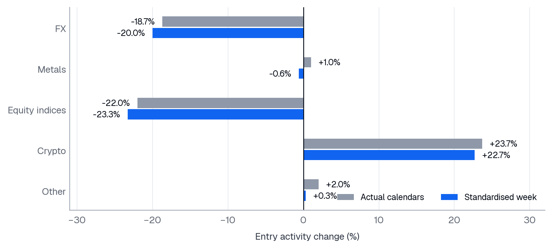
10 July–30 September versus 10 April–30 June. Share and activity-change comparisons answer different questions.
Source: PineConnector Pulse; received instruction aggregates. Shares are instruction-weighted. Download data (CSV): Figure 5
View figure data
| Series | Period | Value | Unit / kind |
|---|---|---|---|
| FX / Actual calendars | Matched available windows | -18.7 | entry activity change %; observed |
| Metals / Actual calendars | Matched available windows | 1.0 | entry activity change %; observed |
| Equity indices / Actual calendars | Matched available windows | -22.0 | entry activity change %; observed |
| Crypto / Actual calendars | Matched available windows | 23.7 | entry activity change %; observed |
| Other / Actual calendars | Matched available windows | 2.0 | entry activity change %; observed |
| FX / Standardised week | Matched available windows | -20.0 | entry activity change %; observed |
| Metals / Standardised week | Matched available windows | -0.6 | entry activity change %; observed |
| Equity indices / Standardised week | Matched available windows | -23.3 | entry activity change %; observed |
| Crypto / Standardised week | Matched available windows | 22.7 | entry activity change %; observed |
| Other / Standardised week | Matched available windows | 0.3 | entry activity change %; observed |
The combined FX-and-metals share increased by 11.7 percentage points between July and September. Equity indices moved from 24.1% to 19.0% and then 17.3% of entries; crypto moved from 13.6% to 12.3% and 10.2%. The consistency is striking, but the monthly mechanisms differed.
In August, FX entry activity rose 28.4% against July and metals rose 15.3%. Equity-index activity fell 14.7% and crypto fell 2.8%. The class rotation therefore combined growing activity on one side with shrinking activity on the other. It was more than a change in shares caused by a moving denominator.
September was different. Total entry activity was approximately unchanged on calendar months, while metals grew 10.6% and FX 2.2%. Equity indices fell 9.1% and crypto 17.0%. Gains and declines substantially offset one another. The flat entry headline concealed a redistribution across markets.
Even the FX result needs a second look. Its three leading published pairs all recorded lower entry activity in September: EUR/USD fell 2.1%, GBP/USD 1.2% and USD/JPY 1.0%. Their combined share of FX activity narrowed from 53.4% to 51.5%. The positive class result therefore came from the remainder of FX activity. A growing category does not imply that its leading components grew.
These are changes in the distribution of instructions. They cannot establish a broad change in preferences or show how widely a pattern was shared. Templates that send instructions frequently can move the aggregate substantially. The evidence establishes the rotation in the received stream; it leaves how widely it was shared and what caused it unresolved.
7. Gold grew while the leading group’s share barely changed
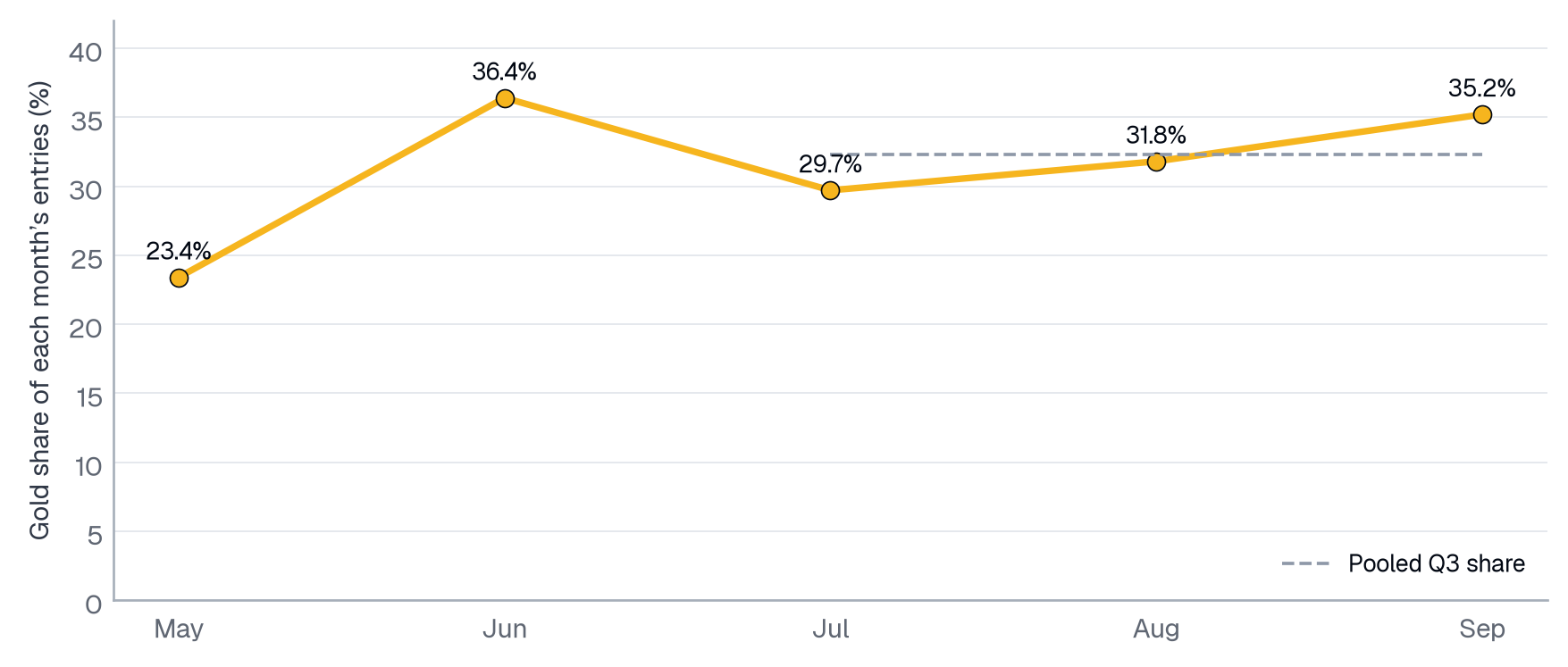
Straight lines connect monthly observations; they are not fitted trends. The dashed reference covers only pooled July–September.
Source: PineConnector Pulse; received instruction aggregates. Shares are instruction-weighted. Download data (CSV): Figure 6
View figure data
| Series | Period | Value | Unit / kind |
|---|---|---|---|
| Gold share | 2026-05 | 23.4 | share of entry instructions %; observed |
| Gold share | 2026-06 | 36.4 | share of entry instructions %; observed |
| Gold share | 2026-07 | 29.7 | share of entry instructions %; observed |
| Gold share | 2026-08 | 31.8 | share of entry instructions %; observed |
| Gold share | 2026-09 | 35.2 | share of entry instructions %; observed |
| Pooled Q3 Gold share | July–September | 32.3 | share of entry instructions %; derived pooled share |
Gold’s entry share rose from 29.7% to 31.8% and 35.2%. Its September activity was 10.8% above August, when it had grown 15.5% against July. Those separate monthly comparisons support the rising-share narrative without constructing a cumulative activity figure.
By September, Gold supplied 99.1% of metals entries. Its entry activity was 97.9% of the entire FX class’s activity. That comparison describes the instruction stream: a single normalised market grouping was nearly as large as the currency class taken together. It does not make Gold’s received instructions equivalent to spot-market transactions.
Yet the four leading markets together took 59.3%, 59.7% and 60.1% of entries. Their combined share changed little. Gold’s growing weight was offset partly within that group: Bitcoin’s share fell from 12.1% to 10.0% between August and September, and Nasdaq 100’s from 7.8% to 7.0%. A rearrangement among leaders can matter even when the leaders’ collective share barely moves.
The class measure tells another story. The effective number of asset classes fell from 3.91 to 3.60 and 3.38. This is the reciprocal of the sum of squared class shares, expressed as the number of equally weighted classes that would produce the same concentration. It measures the balance of activity across classes. The falling value means that balance became more uneven, while the top-market group remained approximately the same size relative to all entries.
Gold’s weekly shares also resist a tidy upward line. Its share reached 39.9% in the full 21–25 September window, then 30.9% in the partial 28–30 September window. The latter covers fewer days and should not be treated as a like-for-like weekly decline. More fundamentally, a weekly share says nothing by itself about whether Gold’s activity level rose: the rest of the entry stream may have contracted faster.
June and September show why the activity-level check matters. Gold’s share rose in both comparisons, but its calendar-month instruction activity fell 16.0% from May to June and rose 10.8% from August to September. The same share direction can accompany opposite activity directions.
8. August became more entry-heavy; September partly reversed it
Entry instructions made up 57.0%, 64.8% and 61.3% of all tracked instructions across the comparable months. The share rose sharply in August and partly retraced in September. It would be misleading to describe the quarter as a steady shift toward entries.
August entries rose 8.1% against July while management-and-other instructions fell 22.0%. Total tracked activity consequently fell 4.8%. September entries were approximately flat on calendar months, while management-and-other activity rose 16.0%, bringing total activity up 5.7%. A fall in entry share can arise because the other instruction group grows, without a corresponding fall in raw entry activity.
The management rebound had a distinct construction. Against August, September pending-order cancellations rose 93.1%, side-specific closes 24.1% and close-all commands 24.2%. SL/TP modification activity fell 31.0% and volume-based partial closes fell 30.1%. Management is not a single activity that scales uniformly. Commands to withdraw or close increased while several adjustment categories declined.
Pending entry activity also rose 23.0% in September, but pending commands represented just 1.7% of entries. Direct-entry shares remained 96.3%, 96.8% and 96.5% through the comparable months. Fast change in a small command family can coexist with a largely unchanged entry-command mix.
The strongest alternative explanation is a change in how instructions were written or routed. An exit can be expressed in the entry message, sent later, or handled through receiving-EA settings. A shift between those arrangements could change management activity without changing the underlying task. Nor do simultaneous increases in pending entries and cancellations link the messages: the aggregates do not establish a lifecycle from placement to withdrawal. The report can identify a changed command mix, not reconstruct the actions behind it.
9. The calendar changed the sign of August’s total comparison
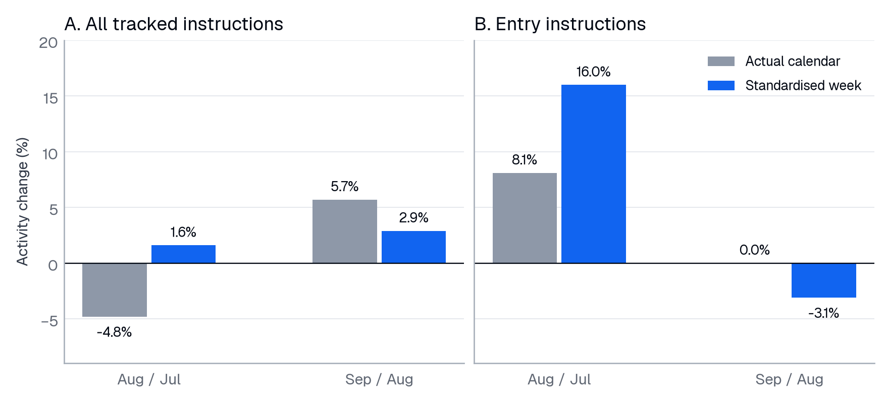
Each month is compared with its predecessor. Standardised-week and calendar-model counterfactual methods are related but distinct.
Source: PineConnector Pulse; received instruction aggregates. Shares are instruction-weighted. Download data (CSV): Figure 7
View figure data
| Series | Period | Value | Unit / kind |
|---|---|---|---|
| Actual calendar | August vs July | -4.8 | activity change %; observed |
| Actual calendar | September vs August | 5.7 | activity change %; observed |
| Standardised week | August vs July | 1.6 | activity change %; observed |
| Standardised week | September vs August | 2.9 | activity change %; observed |
| Actual calendar | August vs July | 8.1 | activity change %; observed |
| Actual calendar | September vs August | 0.0 | activity change %; observed |
| Standardised week | August vs July | 16.0 | activity change %; observed |
| Standardised week | September vs August | -3.1 | activity change %; observed |
August’s raw total decline became a 1.6% increase on a standardised week. Its entry increase became 16.0% on that basis. September’s raw total increase became 2.9%, while its approximately flat entry activity became a 3.1% decline. Calendar composition materially changed the reading in both months.
The standardised week adds each month’s average Monday, average Tuesday and so on through Sunday. It compares the same set of weekday types rather than the actual mix of days in each month. This matters when an average weekend day carries much less entry activity than an average weekday. Dividing everything by calendar days would still leave the weekday mix unresolved.
A separate calendar model asks what September would have looked like if each day had received August’s average activity for the same weekday. For entries, the calendar alone would have produced 3.3% growth; actual activity was approximately flat, leaving a 3.2% decline against that counterfactual. The model and standardised-week comparison therefore tell a similar story: September’s calendar supported entries, masking weaker activity relative to that calendar baseline.
The methods are related sensitivity checks built from the same underlying observations, not independent confirmations. The calendar model assumes the earlier month’s weekday profile can be carried forward. The standardised week can still reflect a quiet holiday or an unusual Monday. Both remove a mechanical calendar difference; neither identifies why instruction activity changed. The model’s residual is a percentage change against its counterfactual, so its components should not be added as if they were percentage points.
10. September’s late decline crossed the published classes
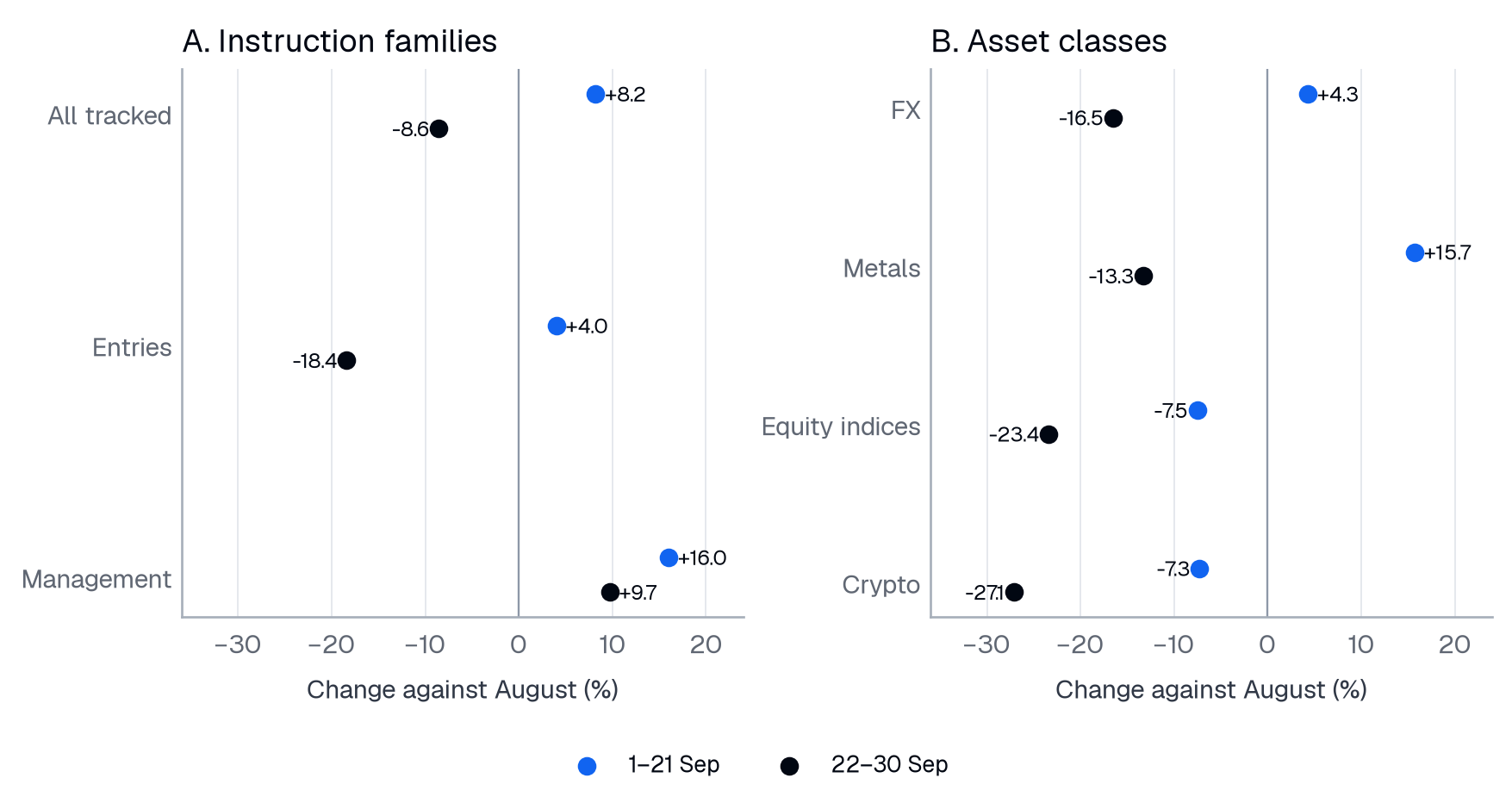
Exploratory split chosen after inspecting September. Both windows compare with all August; late-window values are not changes from the early window.
Source: PineConnector Pulse; received instruction aggregates. Shares are instruction-weighted. Download data (CSV): Figure 8
View figure data
| Series | Period | Value | Unit / kind |
|---|---|---|---|
| All tracked | 1–21 Sep versus all August | 8.2 | standardised activity change %; observed |
| Entries | 1–21 Sep versus all August | 4.0 | standardised activity change %; observed |
| Management | 1–21 Sep versus all August | 16.0 | standardised activity change %; observed |
| All tracked | 22–30 Sep versus all August | -8.6 | standardised activity change %; observed |
| Entries | 22–30 Sep versus all August | -18.4 | standardised activity change %; observed |
| Management | 22–30 Sep versus all August | 9.7 | standardised activity change %; observed |
| FX | 1–21 Sep versus all August | 4.3 | standardised activity change %; observed |
| Metals | 1–21 Sep versus all August | 15.7 | standardised activity change %; observed |
| Equity indices | 1–21 Sep versus all August | -7.5 | standardised activity change %; observed |
| Crypto | 1–21 Sep versus all August | -7.3 | standardised activity change %; observed |
| FX | 22–30 Sep versus all August | -16.5 | standardised activity change %; observed |
| Metals | 22–30 Sep versus all August | -13.3 | standardised activity change %; observed |
| Equity indices | 22–30 Sep versus all August | -23.4 | standardised activity change %; observed |
| Crypto | 22–30 Sep versus all August | -27.1 | standardised activity change %; observed |
The exploratory split makes September’s timeline visible. Entry activity in 1–21 September ran 4.0% above August on a standardised week. In 22–30 September it ran 18.4% below August. Each window is compared with all of August; the late figure is not a percentage change from the first window.
The early window continued the class rotation. Metals were 15.7% above August and FX 4.3% above, while indices were 7.5% below and crypto 7.3% below. Late in the month, all four published class comparisons were negative: FX 16.5%, metals 13.3%, indices 23.4% and crypto 27.1% below August. The late weakness extended beyond the classes already losing activity early in September.
The composition moved much less than those activity comparisons. FX’s entry share shifted from 35.5% to 37.1% between the windows, and metals’ from 35.9% to 34.3%. FX’s share rose while its activity was below the August baseline. That is the denominator mechanism in concrete form: a category can gain relative weight inside a weaker stream.
Several alternative readings can be narrowed. Excluding US Labor Day, 7 September, changes the full-month standardised entry comparison from a 3.1% decline to a 2.7% decline. The difference is small, and the holiday preceded the late window. The last seven weekdays also differed from the limited earlier-month record: their activity was 14.6% above July’s earlier weekdays, 1.4% above August’s, and 22.4% below September’s. Those earlier months offer a useful counterexample to an automatic month-end slowdown, but a thin baseline for a recurring calendar rule.
Management-and-other activity remained 9.7% above August’s standardised baseline in the late window. The received stream was therefore not uniformly weaker across instruction families. This makes a complete cessation of all tracked instruction activity an inadequate explanation. It does not eliminate a disruption or change affecting only part of the entry stream; aggregated management activity could continue elsewhere.
The split date was chosen after inspecting September. It describes the month and should not be presented as a pre-specified breakpoint test. The result also does not tell us whether alert-generation rules changed, some incoming messages stopped arriving, or ordinary activity patterns shifted. A broad class decline is evidence about its scope, not proof of a common cause. That distinction matters more than finding an appealing event to place beside the date.
11. Weekends remained a different stream, and the clock became slightly flatter
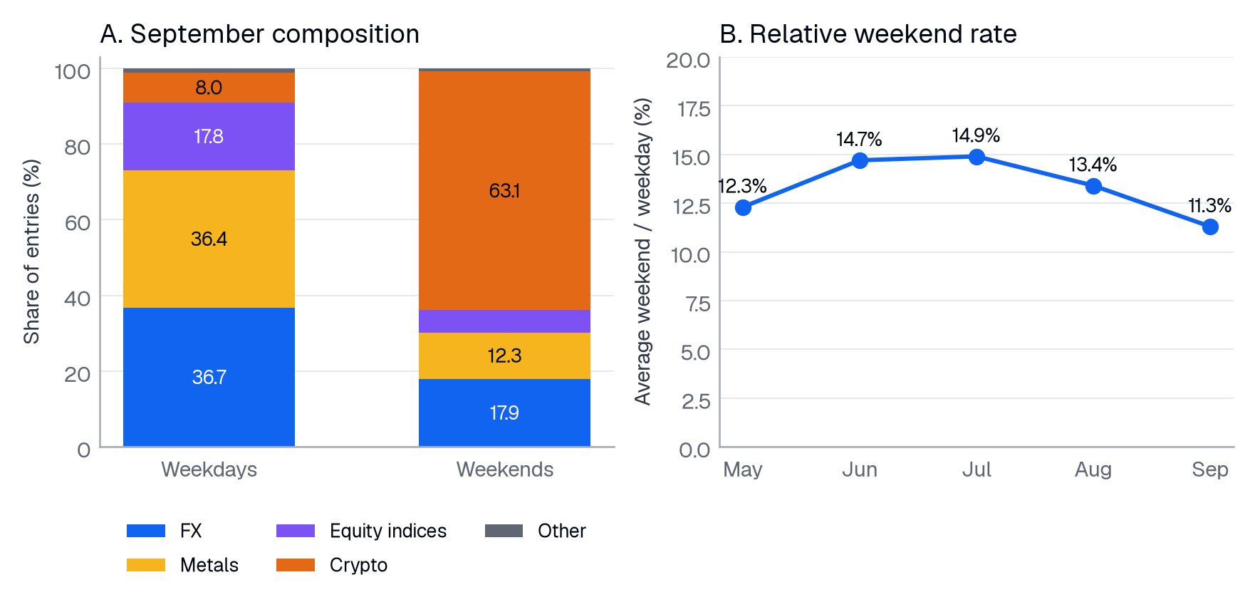
Day types use the source calendar. These figures describe received instructions, not market opening hours or execution schedules.
Source: PineConnector Pulse; received instruction aggregates. Shares are instruction-weighted. Download data (CSV): Figure 9
View figure data
| Series | Period | Value | Unit / kind |
|---|---|---|---|
| FX | September weekdays | 36.7 | share of entry instructions %; observed |
| FX | September weekends | 17.9 | share of entry instructions %; observed |
| Metals | September weekdays | 36.4 | share of entry instructions %; observed |
| Metals | September weekends | 12.3 | share of entry instructions %; observed |
| Equity indices | September weekdays | 17.8 | share of entry instructions %; observed |
| Equity indices | September weekends | 5.9 | share of entry instructions %; observed |
| Crypto | September weekdays | 8.0 | share of entry instructions %; observed |
| Crypto | September weekends | 63.1 | share of entry instructions %; observed |
| Other | September weekdays | 1.1 | share of entry instructions %; observed |
| Other | September weekends | 0.8 | share of entry instructions %; observed |
| Weekend / weekday rate | 2026-05 | 12.3 | average day rate ratio %; observed |
| Weekend / weekday rate | 2026-06 | 14.7 | average day rate ratio %; observed |
| Weekend / weekday rate | 2026-07 | 14.9 | average day rate ratio %; observed |
| Weekend / weekday rate | 2026-08 | 13.4 | average day rate ratio %; observed |
| Weekend / weekday rate | 2026-09 | 11.3 | average day rate ratio %; observed |
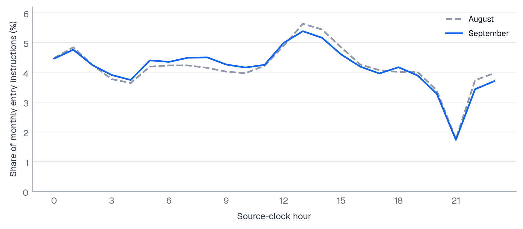
Pooled monthly distribution by hour, not a chronological intraday series. The source timezone is unconfirmed; no UTC, SGT or event-time alignment is inferred.
Source: PineConnector Pulse; received instruction aggregates. Shares are instruction-weighted. Download data (CSV): Figure 10
View figure data
| Series | Period | Value | Unit / kind |
|---|---|---|---|
| August | 00:00 source clock | 4.48 | share of month entries %; observed |
| August | 01:00 source clock | 4.84 | share of month entries %; observed |
| August | 02:00 source clock | 4.25 | share of month entries %; observed |
| August | 03:00 source clock | 3.77 | share of month entries %; observed |
| August | 04:00 source clock | 3.64 | share of month entries %; observed |
| August | 05:00 source clock | 4.19 | share of month entries %; observed |
| August | 06:00 source clock | 4.23 | share of month entries %; observed |
| August | 07:00 source clock | 4.23 | share of month entries %; observed |
| August | 08:00 source clock | 4.15 | share of month entries %; observed |
| August | 09:00 source clock | 4.02 | share of month entries %; observed |
| August | 10:00 source clock | 3.97 | share of month entries %; observed |
| August | 11:00 source clock | 4.22 | share of month entries %; observed |
| August | 12:00 source clock | 4.89 | share of month entries %; observed |
| August | 13:00 source clock | 5.63 | share of month entries %; observed |
| August | 14:00 source clock | 5.44 | share of month entries %; observed |
| August | 15:00 source clock | 4.84 | share of month entries %; observed |
| August | 16:00 source clock | 4.26 | share of month entries %; observed |
| August | 17:00 source clock | 4.07 | share of month entries %; observed |
| August | 18:00 source clock | 4.01 | share of month entries %; observed |
| August | 19:00 source clock | 4.01 | share of month entries %; observed |
| August | 20:00 source clock | 3.39 | share of month entries %; observed |
| August | 21:00 source clock | 1.76 | share of month entries %; observed |
| August | 22:00 source clock | 3.73 | share of month entries %; observed |
| August | 23:00 source clock | 3.97 | share of month entries %; observed |
| September | 00:00 source clock | 4.46 | share of month entries %; observed |
| September | 01:00 source clock | 4.76 | share of month entries %; observed |
| September | 02:00 source clock | 4.24 | share of month entries %; observed |
| September | 03:00 source clock | 3.91 | share of month entries %; observed |
| September | 04:00 source clock | 3.74 | share of month entries %; observed |
| September | 05:00 source clock | 4.4 | share of month entries %; observed |
| September | 06:00 source clock | 4.35 | share of month entries %; observed |
| September | 07:00 source clock | 4.49 | share of month entries %; observed |
| September | 08:00 source clock | 4.5 | share of month entries %; observed |
| September | 09:00 source clock | 4.26 | share of month entries %; observed |
| September | 10:00 source clock | 4.16 | share of month entries %; observed |
| September | 11:00 source clock | 4.25 | share of month entries %; observed |
| September | 12:00 source clock | 4.99 | share of month entries %; observed |
| September | 13:00 source clock | 5.38 | share of month entries %; observed |
| September | 14:00 source clock | 5.16 | share of month entries %; observed |
| September | 15:00 source clock | 4.6 | share of month entries %; observed |
| September | 16:00 source clock | 4.19 | share of month entries %; observed |
| September | 17:00 source clock | 3.96 | share of month entries %; observed |
| September | 18:00 source clock | 4.17 | share of month entries %; observed |
| September | 19:00 source clock | 3.89 | share of month entries %; observed |
| September | 20:00 source clock | 3.28 | share of month entries %; observed |
| September | 21:00 source clock | 1.73 | share of month entries %; observed |
| September | 22:00 source clock | 3.43 | share of month entries %; observed |
| September | 23:00 source clock | 3.7 | share of month entries %; observed |
An average weekend day’s entries were 14.9%, 13.4% and 11.3% of an average weekday’s across the comparable months. Crypto’s share of weekend entries narrowed from 72.3% to 67.7% and 63.1%. By September, crypto still made up most weekend activity while accounting for 8.0% of weekday entries. Gold supplied 36.1% of weekday entries and 12.2% of weekend entries.
A declining monthly crypto share is consistent with a smaller weekend relative to weekdays because crypto’s instruction activity is much more evenly distributed across day types. But this cannot be attributed to class weights alone. Crypto’s own average weekend-day activity moved from 104.5% to 89.5% of its average weekday activity between August and September. Both the class mix and the rhythm within crypto changed.
The aggregate peak-to-quiet hourly ratio eased from 3.32× to 3.20× and 3.11×. September’s strongest source-clock block, 12:00-15:59, contained 20.1% of entries. Metals had a much more uneven hourly distribution than FX or crypto: their September peak-to-quiet ratios were 28.65×, 1.37× and 1.18×, respectively. Those differences help explain why a platform average combines quite different rhythms.
They do not justify saying that Gold’s rising share made the platform’s peaks sharper. The observed aggregate ratio moved the other way. Metals’ own hourly ratio also fell from 61.98× in August. Class weights and within-class timing can push against each other, and their busiest hours need not coincide. The class-rhythm figure is for metals; it should not be relabelled as an exact Gold-only curve.
The source timezone remains unconfirmed. These are distributions on the source clock, not precise alignments with Singapore time, a market session or an announcement. Weekend instructions can arrive when an underlying market is closed. The figures describe when requests reached the bridge, not a schedule for execution.
12. Exit-field construction changed inside classes
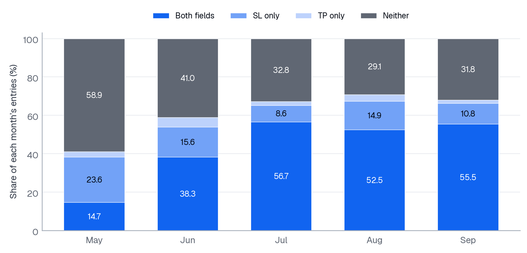
Field presence does not establish field validity, broker acceptance or protection. Displayed partitions are independently rounded.
Source: PineConnector Pulse; received instruction aggregates. Shares are instruction-weighted. Download data (CSV): Figure 11
View figure data
| Series | Period | Value | Unit / kind |
|---|---|---|---|
| Both fields | 2026-05 | 14.7 | share of entry instructions %; observed |
| Both fields | 2026-06 | 38.3 | share of entry instructions %; observed |
| Both fields | 2026-07 | 56.7 | share of entry instructions %; observed |
| Both fields | 2026-08 | 52.5 | share of entry instructions %; observed |
| Both fields | 2026-09 | 55.5 | share of entry instructions %; observed |
| SL only | 2026-05 | 23.6 | share of entry instructions %; observed |
| SL only | 2026-06 | 15.6 | share of entry instructions %; observed |
| SL only | 2026-07 | 8.6 | share of entry instructions %; observed |
| SL only | 2026-08 | 14.9 | share of entry instructions %; observed |
| SL only | 2026-09 | 10.8 | share of entry instructions %; observed |
| TP only | 2026-05 | 2.8 | share of entry instructions %; observed |
| TP only | 2026-06 | 5.0 | share of entry instructions %; observed |
| TP only | 2026-07 | 1.9 | share of entry instructions %; observed |
| TP only | 2026-08 | 3.5 | share of entry instructions %; observed |
| TP only | 2026-09 | 1.8 | share of entry instructions %; observed |
| Neither | 2026-05 | 58.9 | share of entry instructions %; observed |
| Neither | 2026-06 | 41.0 | share of entry instructions %; observed |
| Neither | 2026-07 | 32.8 | share of entry instructions %; observed |
| Neither | 2026-08 | 29.1 | share of entry instructions %; observed |
| Neither | 2026-09 | 31.8 | share of entry instructions %; observed |
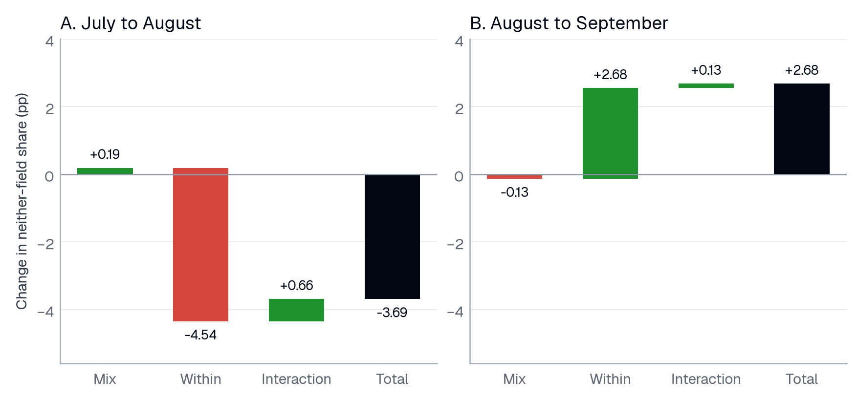
Accounting decomposition, not a causal attribution. Components sum to the source-published total at its displayed precision.
Source: PineConnector Pulse; received instruction aggregates. Shares are instruction-weighted. Download data (CSV): Figure 12
View figure data
| Series | Period | Value | Unit / kind |
|---|---|---|---|
| Mix | july_to_august | 0.19 | percentage points; observed |
| Within | july_to_august | -4.54 | percentage points; observed |
| Interaction | july_to_august | 0.66 | percentage points; observed |
| Total | july_to_august | -3.69 | percentage points; derived share change |
| Mix | august_to_september | -0.13 | percentage points; observed |
| Within | august_to_september | 2.68 | percentage points; observed |
| Interaction | august_to_september | 0.13 | percentage points; observed |
| Total | august_to_september | 2.68 | percentage points; derived share change |
The complete-month sequence supplies a longer context: the neither-field share was 58.9% in May and 41.0% in June before the lower Q3 levels shown below. This is a change in recognised instruction fields, not proof that exit arrangements changed at the broker.
Comparable entries carrying neither recognised SL nor TP field represented 32.8%, 29.1% and 31.8% across the months. Like the entry/management split, the measure moved one way in August and partly back in September. It describes the message as received; it does not establish whether an exit was configured elsewhere.
September’s four-way partition is revealing. Entries carrying both recognised fields increased to 55.5%, while SL-only entries fell to 10.8% and TP-only entries to 1.8%. The neither-field group also increased. Consequently, any recognised SL presence fell by 0.9 percentage points to 66.4%, even as any recognised TP presence rose by 1.4 percentage points to 57.4%. The increase in the both-field group cannot stand in for the whole construction story. Each published rate is rounded independently, so adding displayed groups can differ slightly from the separately published derived rate.
Could the class rotation explain the platform’s neither-field change? September’s approved shift-share decomposition assigns -0.13 percentage points to changing class weights, +2.68 percentage points to changes within classes and +0.13 percentage points to their interaction, for a total +2.68 percentage points change. The mix effect was small and pointed against the overall increase. Within-class change was the dominant component.
July to August showed the same distinction with the overall movement reversed: -3.69 percentage points in total, comprising +0.19 percentage points from the mix, -4.54 percentage points within classes and +0.66 percentage points from the interaction. The large market rotation did not mechanically explain the field-profile movement in either comparison.
The decomposition changes one element at a time. Its mix term moves the class weights while holding the earlier field rates fixed. Its within term changes those rates while holding earlier weights fixed. The interaction records the joint movement. This is an accounting identity, not evidence that each component represents a separate causal process.
Metals’ neither-field share rose 6.7 percentage points in September and contributed +2.16 percentage points to the platform’s within-class movement. Indices moved the other way: their neither-field share fell 2.4 percentage points, while recognised TP presence rose 9.8 percentage points. A single platform average hides those opposing changes.
Here, the strongest alternative to a change in exit practice is a change in instruction templates within a class. Different templates can carry different fields, and exits may be handled through EA settings or later messages. A within-class effect does not hold those templates constant. It rules out class weighting as the main arithmetic explanation; it cannot establish that unchanged templates altered their construction. Recognised field presence also does not prove valid levels, broker acceptance or protection.
13. The market backdrop: a flat dollar headline hid a round trip
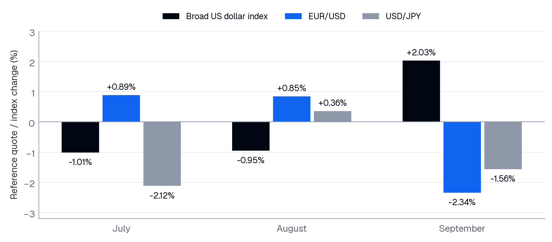
External Federal Reserve H.10 references only. Changes use prior month-end to current month-end; they are quote/index changes, not investment returns or PineConnector activity.
Source: Federal Reserve H.10 Download data (CSV): Figure 13
View figure data
| Series | Period | Value | Unit / kind |
|---|---|---|---|
| Broad US dollar index | July | -1.01 | external reference change %; observed |
| Broad US dollar index | August | -0.95 | external reference change %; observed |
| Broad US dollar index | September | 2.03 | external reference change %; observed |
| EUR/USD | July | 0.89 | external reference change %; observed |
| EUR/USD | August | 0.85 | external reference change %; observed |
| EUR/USD | September | -2.34 | external reference change %; observed |
| USD/JPY | July | -2.12 | external reference change %; observed |
| USD/JPY | August | 0.36 | external reference change %; observed |
| USD/JPY | September | -1.56 | external reference change %; observed |
The external market record supplies a real Q2-to-Q3 comparison, but it answers a different question from the instruction record. Federal Reserve H.10 reference rates show where currencies and the broad dollar index stood at each quarter boundary. They do not show PineConnector activity, execution or trading outcomes.
The broad dollar index was nearly unchanged over both quarters: -0.09% in Q2 and +0.04% in Q3. The route through Q3 was much less flat. It fell -1.01% in July and -0.95% in August, then rose +2.03% in September, finishing near its June boundary. A quiet quarter-end comparison therefore concealed two declining months followed by a reversal.
| External reference series | Q2 change | Q3 change | July | August | September |
|---|---|---|---|---|---|
| EUR/USD | -0.88% | -0.63% | +0.89% | +0.85% | -2.34% |
| USD/JPY | +2.22% | -3.30% | -2.12% | +0.36% | -1.56% |
| GBP/USD | +0.57% | +0.06% | +1.59% | +0.59% | -2.09% |
| USD/SGD | +0.37% | -1.31% | -0.87% | -0.86% | +0.42% |
| Broad US dollar index | -0.09% | +0.04% | -1.01% | -0.95% | +2.03% |
Changes are calculated as 100 × (end reference / start reference − 1). Q2 uses 31 March to 30 June; Q3 uses 30 June to 30 September. Monthly figures use the previous month-end reference. Each figure is calculated directly from its endpoints, rather than by adding rounded monthly changes. EUR/USD and GBP/USD are US dollars per euro and pound; USD/JPY and USD/SGD are yen and Singapore dollars per US dollar. A negative USD/JPY change means fewer yen per dollar. The table reports quote/index changes, not investment returns.
USD/JPY changed direction across quarters: +2.22% in Q2 and -3.30% in Q3. EUR/USD ended both quarters lower, but that headline hid a different Q3 path: increases in July and August, then a September decline. The broad dollar index and individual pairs therefore give different views of the same period. A single dollar headline cannot represent every FX market.
This backdrop makes the internal FX finding more interesting without explaining it. The FX class gained instruction share across the comparable Q3 observations, while its three leading published pairs each recorded lower instruction activity in September. The external September reversal and the internal redistribution are separate observations. The available records do not identify whether one produced the other.
Sources: Federal Reserve H.10 releases on 6 April, 6 July, 3 August, 8 September and 5 October 2026, accessed 11 October 2026. These are reference observations and can be revised. The full-quarter external table is separate from the monthly Pulse comparisons; it is not a Q2-to-Q3 PineConnector instruction comparison.
14. Q4 conditional outlook: month and quarter sensitivity
These scenarios were prepared on 11 October 2026, using instruction data ending 30 September. October was already underway, but no October observations are incorporated. The paths are full-month conditional illustrations, not an October nowcast; they have not been statistically validated. Dashed lines denote assumptions. They have no assigned probabilities, and the space between them is not a confidence interval.
Activity cases anchored to September
The carry-forward benchmark keeps September’s mean entry activity for each weekday. The first-window-return case moves October’s average level halfway from the whole-September standardised rate to the 1–21 September rate, then uses the first-window rate in November and December. “Halfway” means a level midpoint across all October days; it is not a first-half/second-half month split. The late-window-persistence case applies the 22–30 September standardised rate in each Q4 month. Both window anchors were chosen after inspecting September and are sensitivity inputs, not demonstrated regimes.
The calendar step applies the September entry-specific weekday rates to each future month. No holiday-specific adjustment is made. September’s rates already reflect its holiday and month-end pattern; the model neither estimates Thanksgiving/year-end effects nor removes those embedded September influences. A December increase can therefore be a weekday-count result, not a claim that December will be stronger in practice.
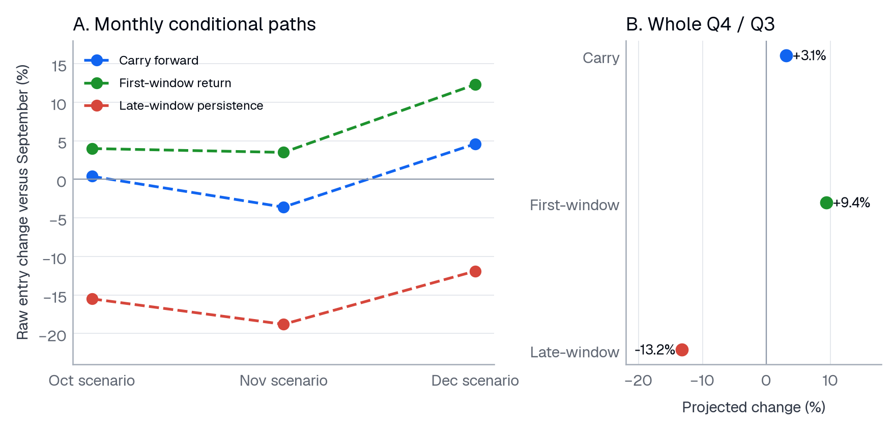
Illustrative scenarios prepared 11 October using activity through 30 September. October actuals are not used. No probabilities, calibrated uncertainty intervals or holiday-specific adjustment. Quarter changes are calculated from summed projected activity, not average monthly changes.
Source: PineConnector Pulse conditional calculations; assumptions stated in the Q4 section. Download data (CSV): Figure 14
View figure data
| Series | Period | Value | Unit / kind |
|---|---|---|---|
| Carry forward | October | 0.4 | projected activity change vs September %; conditional scenario |
| Carry forward | November | -3.6 | projected activity change vs September %; conditional scenario |
| Carry forward | December | 4.6 | projected activity change vs September %; conditional scenario |
| Carry forward | Q4 versus complete Q3 | 3.1 | projected activity change %; conditional scenario |
| First-window return | October | 4.0 | projected activity change vs September %; conditional scenario |
| First-window return | November | 3.5 | projected activity change vs September %; conditional scenario |
| First-window return | December | 12.3 | projected activity change vs September %; conditional scenario |
| First-window return | Q4 versus complete Q3 | 9.4 | projected activity change %; conditional scenario |
| Late-window persistence | October | -15.5 | projected activity change vs September %; conditional scenario |
| Late-window persistence | November | -18.8 | projected activity change vs September %; conditional scenario |
| Late-window persistence | December | -11.9 | projected activity change vs September %; conditional scenario |
| Late-window persistence | Q4 versus complete Q3 | -13.2 | projected activity change %; conditional scenario |
| Conditional entry-activity case | October / September | November / September | December / September | Q4 / whole Q3 |
|---|---|---|---|---|
| Carry September weekday rates | +0.4% | -3.6% | +4.6% | +3.1% |
| Return to first-window level | +4.0% | +3.5% | +12.3% | +9.4% |
| Persist at late-window level | -15.5% | -18.8% | -11.9% | -13.2% |
The monthly columns compare projected raw entry activity with complete September. The quarter column compares summed projected Q4 activity with the underlying full-Q3 aggregates. Their baselines differ, so neither a simple average of the monthly percentages nor chaining rounded source percentages produces the quarter result. All projected levels remain undisclosed. With weekday-specific activity unchanged, the standardised-week change is flat even when the calendar-month totals differ.
Composition paths are a separate exercise
The composition panel asks a different question: what would Gold’s instruction share look like if the September mix held, moved halfway toward the pooled Q3 mix in October and reached it from November, or continued the July-to-September Gold-share slope mechanically? In the slope case, the extra Gold share is assigned to metals; other classes are reduced proportionately and the residual non-Gold metals share is held fixed. These rules keep all shares bounded and the class whole coherent. Rounded historical anchors are normalized only for this hypothetical arithmetic; observed tables retain their published values.
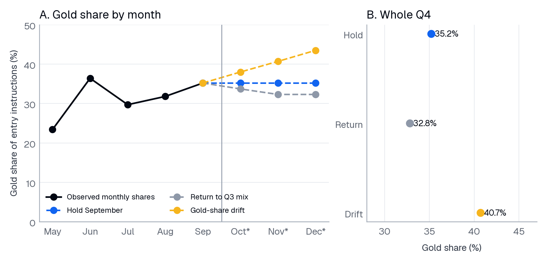
Starred months are hypothetical. Mix paths are separate from the activity cases; whole-Q4 mix uses calendar-only projected activity weights. Rounded historical anchors are normalized only for scenario arithmetic. Scope: received instruction shares only.
Source: PineConnector Pulse conditional calculations; assumptions stated in the Q4 section. Download data (CSV): Figure 15
View figure data
| Series | Period | Value | Unit / kind |
|---|---|---|---|
| Observed Gold share | 2026-05 | 23.4 | share of entry instructions %; observed |
| Observed Gold share | 2026-06 | 36.4 | share of entry instructions %; observed |
| Observed Gold share | 2026-07 | 29.7 | share of entry instructions %; observed |
| Observed Gold share | 2026-08 | 31.8 | share of entry instructions %; observed |
| Observed Gold share | 2026-09 | 35.2 | share of entry instructions %; observed |
| Hold September | October | 35.2 | projected Gold entry share %; conditional sensitivity |
| Hold September | November | 35.2 | projected Gold entry share %; conditional sensitivity |
| Hold September | December | 35.2 | projected Gold entry share %; conditional sensitivity |
| Return to Q3 mix | October | 33.7 | projected Gold entry share %; conditional sensitivity |
| Return to Q3 mix | November | 32.3 | projected Gold entry share %; conditional sensitivity |
| Return to Q3 mix | December | 32.3 | projected Gold entry share %; conditional sensitivity |
| Gold-share drift | October | 38.0 | projected Gold entry share %; conditional sensitivity |
| Gold-share drift | November | 40.7 | projected Gold entry share %; conditional sensitivity |
| Gold-share drift | December | 43.5 | projected Gold entry share %; conditional sensitivity |
| Hold September | Whole Q4 | 35.2 | projected Gold entry share %; conditional sensitivity |
| Return to Q3 mix | Whole Q4 | 32.8 | projected Gold entry share %; conditional sensitivity |
| Gold-share drift | Whole Q4 | 40.7 | projected Gold entry share %; conditional sensitivity |
| Gold-share sensitivity | October | November | December | Whole Q4 |
|---|---|---|---|---|
| Hold September mix | 35.2% | 35.2% | 35.2% | 35.2% |
| Return to pooled Q3 mix | 33.7% | 32.3% | 32.3% | 32.8% |
| Continue Gold-share slope | 38.0% | 40.7% | 43.5% | 40.7% |
Whole-Q4 composition uses calendar-only projected entry-activity weights. This panel is independent of the activity cases; it is not a joint model coupling Gold share and aggregate activity. The composition paths concern received instruction shares.
What would change the outlook
The carry-forward case would lose usefulness if the next completed month’s weekday-standardised entry rate moved materially away from September’s. A return toward the first-window rate would support that conditional case; sustained weakness near the late-window rate would support persistence. Each comparison must use the same eligibility and source-clock definitions and a complete month. Partial October readings cannot be scored directly against full-month paths.
For composition, a rise beyond June’s Gold share would change the “recovery within Q3” interpretation; renewed broadening toward indices or crypto would challenge the continuation of the September mix. These are proposed tests prepared on 11 October; success cannot be assessed before future observations arrive. Future observations should be checked against the saved assumptions and reported with their actual dates, including results that contradict the appealing case.
Method reference: Hyndman and Athanasopoulos, Forecasting: Principles and Practice, scenario construction.
15. Q4 enters with inflation constraints and uneven growth
This external outlook is prepared on 11 October 2026. It uses public economic releases and institutional projections available at that date, including releases issued after Q3 ended. The PineConnector instruction dataset still ends on 30 September. The two evidence sets have different cutoffs and remain separate: external conditions provide hypotheses to examine, not coefficients for the instruction scenarios or evidence of a price response caused by PineConnector activity.
The central tension is an economy that can keep expanding while inflation restricts policy flexibility. The IMF’s July update put global full-year growth at 3.0% in 2026 and 3.4% in 2027, with energy disruption and technology investment pulling in different directions. Those annual projections supply background, not a Q4 growth rate. We retain that July vintage rather than assuming a later IMF update is already available. IMF, July 2026 World Economic Outlook update.
Policy entered Q4 with renewed tightening
The Federal Reserve raised its target range to 3.75–4.00% on 16 September. The ECB raised its deposit-facility rate to 2.50%, effective 16 September. The Bank of Japan’s 18 September guideline set the overnight call rate at around 1.25%. These are different policy instruments and conventions; their levels do not by themselves establish equivalent restrictiveness across economies. Fed statement; ECB decision; BoJ guideline.
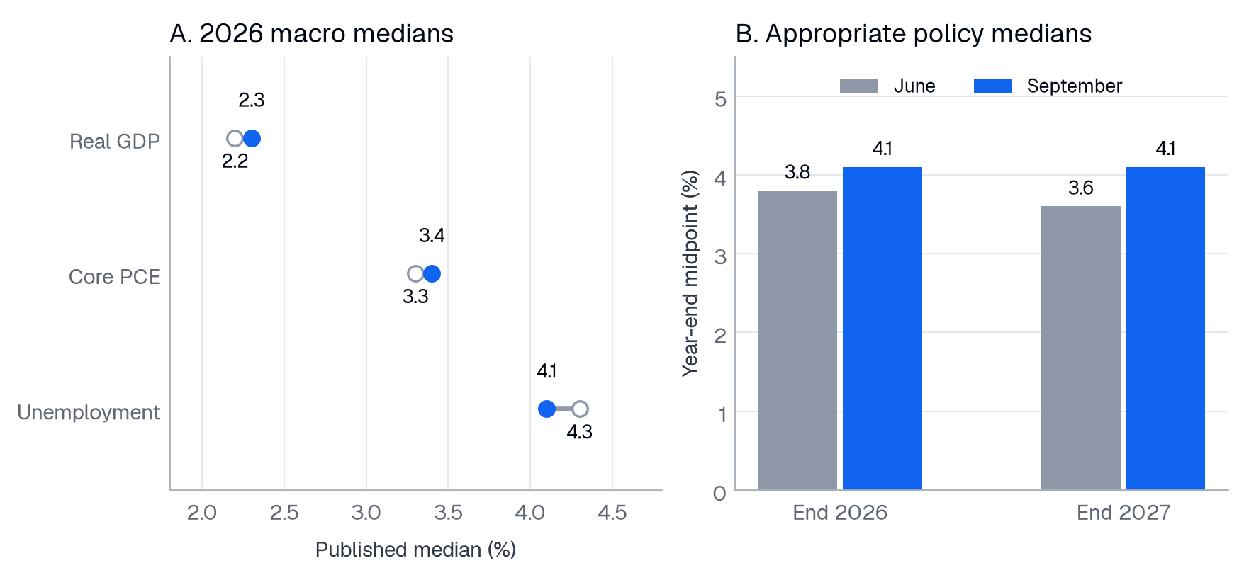
June versus September 2026 SEP medians. Panel A: GDP and core PCE use Q4/Q4 changes; unemployment is a Q4 average. Open markers: June; blue: September. Panel B: year-end appropriate policy midpoints. Conditional participant views, not policy commitments or market odds. External evidence only.
Source: Federal Reserve, September 2026 Summary of Economic Projections Download data (CSV): Figure 16
View figure data
| Series | Period | Value | Unit / kind |
|---|---|---|---|
| Real GDP | 2026 / June projection | 2.2 | Q4/Q4 real GDP change %; institutional projection |
| Real GDP | 2026 / September projection | 2.3 | Q4/Q4 real GDP change %; institutional projection |
| Core PCE | 2026 / June projection | 3.3 | Q4/Q4 core PCE price change %; institutional projection |
| Core PCE | 2026 / September projection | 3.4 | Q4/Q4 core PCE price change %; institutional projection |
| Unemployment | 2026 / June projection | 4.3 | Q4 average civilian unemployment %; institutional projection |
| Unemployment | 2026 / September projection | 4.1 | Q4 average civilian unemployment %; institutional projection |
| Appropriate federal funds midpoint | 2026 year-end / June projection | 3.8 | year-end appropriate policy midpoint %; institutional projection |
| Appropriate federal funds midpoint | 2027 year-end / June projection | 3.6 | year-end appropriate policy midpoint %; institutional projection |
| Appropriate federal funds midpoint | 2026 year-end / September projection | 4.1 | year-end appropriate policy midpoint %; institutional projection |
| Appropriate federal funds midpoint | 2027 year-end / September projection | 4.1 | year-end appropriate policy midpoint %; institutional projection |
The Fed’s September medians shifted toward stronger 2026 growth, higher core inflation and lower Q4 unemployment than in June. The appropriate year-end policy median also rose for both displayed years. This makes a simple assumption of immediate easing a weak starting point. These are participants’ conditional views of appropriate policy, not promised decisions or market-implied odds. GDP and inflation use Q4-to-Q4 changes; unemployment is a Q4 average; the policy rate is a year-end midpoint. None is Q4 quarter-on-quarter growth. September SEP, Table 1.
Softer hiring complicates the inflation story
The 2 October jobs release reported a September payroll increase of 29,000, unemployment of 4.2%, and combined downward revisions of 60,000 to July and August job gains. Payroll changes are seasonally adjusted. A weak month and revisions warrant attention, but do not alone establish a recession. BLS September jobs release.
The latest CPI release inspected here covers August: headline CPI-U rose 3.4% over twelve months and CPI excluding food and energy rose 2.4%, both before seasonal adjustment. CPI and the Fed’s projected PCE measure use different price baskets and reference periods; they should not be read as a direct observed-versus-projected scorecard. BLS August CPI release.
For Europe, the ECB staff baseline places HICP inflation at 3.6% in Q4 2026, a year-on-year rate shaped by energy pressures. Its alternative scenarios illustrate how the duration of that shock can change the following year. Figure 17 deliberately shows 2027 annual outcomes, not Q4 2026 estimates. ECB September projections, overview and Box 4.
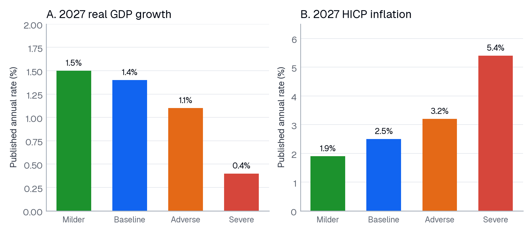
ECB September 2026 projections, Box 4 Table C. These are 2027 annual outcomes under the ECB’s named energy-shock cases, not Q4 2026 growth or inflation. Values re-tabulated without adjustment; no probabilities inferred.
Source: ECB staff, September 2026 macroeconomic projections Download data (CSV): Figure 17
View figure data
| Series | Period | Value | Unit / kind |
|---|---|---|---|
| Milder | 2027 annual | 1.5 | annual real GDP growth %; institutional conditional scenario |
| Baseline | 2027 annual | 1.4 | annual real GDP growth %; institutional conditional scenario |
| Adverse | 2027 annual | 1.1 | annual real GDP growth %; institutional conditional scenario |
| Severe | 2027 annual | 0.4 | annual real GDP growth %; institutional conditional scenario |
| Milder | 2027 annual | 1.9 | annual-average HICP inflation %; institutional conditional scenario |
| Baseline | 2027 annual | 2.5 | annual-average HICP inflation %; institutional conditional scenario |
| Adverse | 2027 annual | 3.2 | annual-average HICP inflation %; institutional conditional scenario |
| Severe | 2027 annual | 5.4 | annual-average HICP inflation %; institutional conditional scenario |
The implication for this paper is a conditional one: an energy shock can constrain household purchasing power and business margins while raising measured inflation. A central bank responding to that inflation may face a different choice from one confronting a pure demand slowdown. One generic “risk” label therefore hides mechanisms that can pull asset prices in opposing directions.
16. October, November and December pose different tests
The calendar is a map of selected future checkpoints, checked on 11 October, rather than a complete release schedule. Dates below are the issuing institution’s local calendar dates. A two-day meeting spans both dates; the plot marks its final day. Scheduled events can change. Their presence does not establish the size or direction of a market move, and the source-clock uncertainty prevents aligning PineConnector instructions with them as an event study.
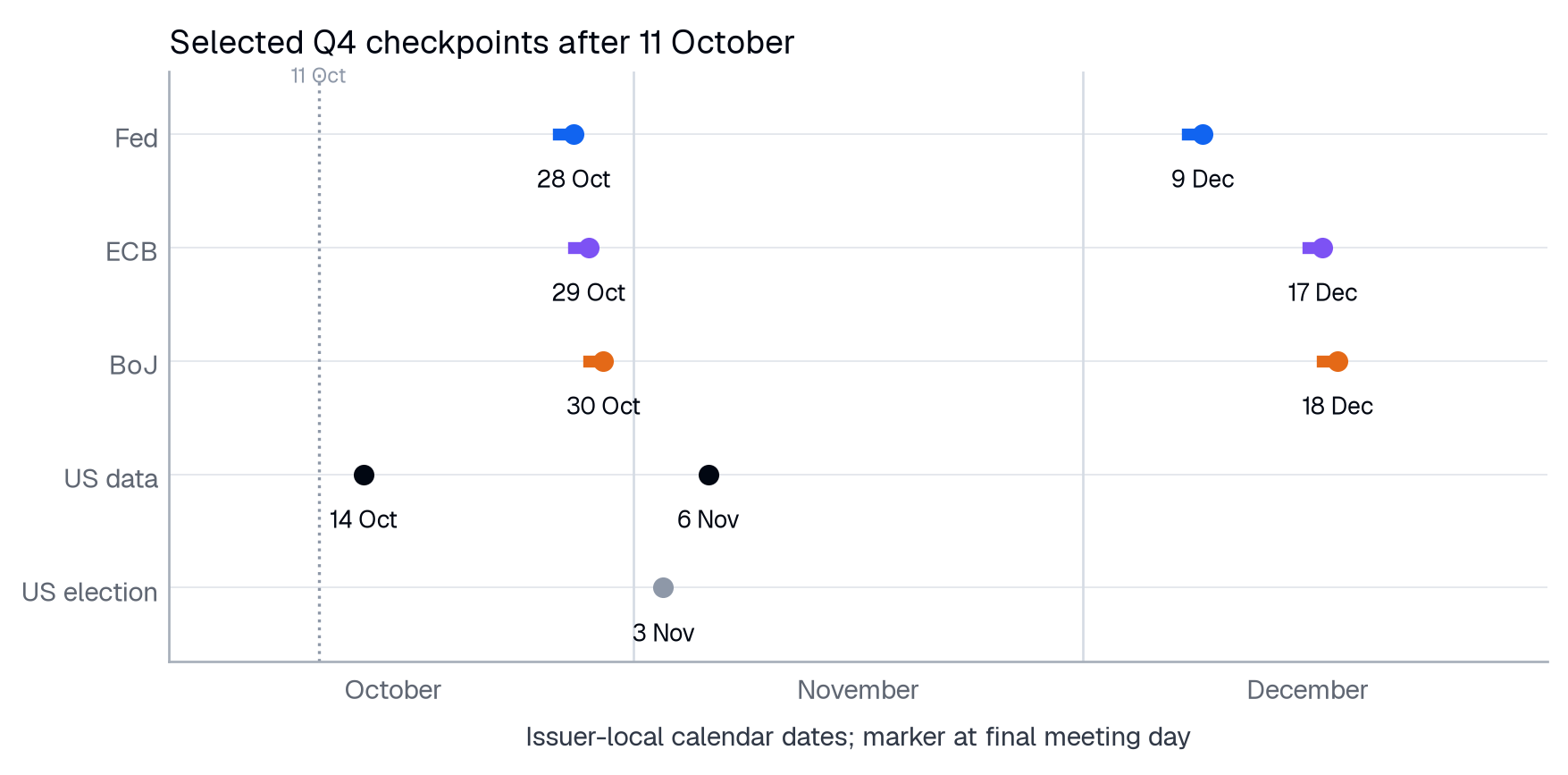
Selected schedule checked 11 October; not a complete calendar. Spans show full two-day meetings; labels show their final day. US data: CPI on 14 October and jobs on 6 November. US election: 3 November. Dates may change; no market response or source-clock alignment inferred.
Source: Federal Reserve, 2026 FOMC calendar; ECB, Governing Council calendar; Bank of Japan, 2026 meeting schedule; BLS, August 2026 Consumer Price Index; BLS, September 2026 Employment Situation; FEC, 2026 general-election dates Download data (CSV): Figure 18
View figure data
| Series | Period | Value | Unit / kind |
|---|---|---|---|
| US data / September CPI / start | 2026-10-14 | 13 | calendar days since 2026-10-01; scheduled date metadata |
| US data / September CPI / end | 2026-10-14 | 13 | calendar days since 2026-10-01; scheduled date metadata |
| Fed / FOMC / start | 2026-10-27 | 26 | calendar days since 2026-10-01; scheduled date metadata |
| Fed / FOMC / end | 2026-10-28 | 27 | calendar days since 2026-10-01; scheduled date metadata |
| ECB / Policy meeting / start | 2026-10-28 | 27 | calendar days since 2026-10-01; scheduled date metadata |
| ECB / Policy meeting / end | 2026-10-29 | 28 | calendar days since 2026-10-01; scheduled date metadata |
| BoJ / MPM / outlook / start | 2026-10-29 | 28 | calendar days since 2026-10-01; scheduled date metadata |
| BoJ / MPM / outlook / end | 2026-10-30 | 29 | calendar days since 2026-10-01; scheduled date metadata |
| US election / General election / start | 2026-11-03 | 33 | calendar days since 2026-10-01; scheduled date metadata |
| US election / General election / end | 2026-11-03 | 33 | calendar days since 2026-10-01; scheduled date metadata |
| US data / October jobs / start | 2026-11-06 | 36 | calendar days since 2026-10-01; scheduled date metadata |
| US data / October jobs / end | 2026-11-06 | 36 | calendar days since 2026-10-01; scheduled date metadata |
| Fed / FOMC / SEP / start | 2026-12-08 | 68 | calendar days since 2026-10-01; scheduled date metadata |
| Fed / FOMC / SEP / end | 2026-12-09 | 69 | calendar days since 2026-10-01; scheduled date metadata |
| ECB / Policy meeting / start | 2026-12-16 | 76 | calendar days since 2026-10-01; scheduled date metadata |
| ECB / Policy meeting / end | 2026-12-17 | 77 | calendar days since 2026-10-01; scheduled date metadata |
| BoJ / MPM / start | 2026-12-17 | 77 | calendar days since 2026-10-01; scheduled date metadata |
| BoJ / MPM / end | 2026-12-18 | 78 | calendar days since 2026-10-01; scheduled date metadata |
October: test inflation before the policy cluster
September CPI is scheduled for 14 October. The FOMC meets on 27–28 October, the ECB on 28–29 October, and the BoJ on 29–30 October, with the latter also scheduled to issue an outlook. The sequence offers a practical test of whether inflation pressure is broadening, easing or remaining concentrated in energy. A fresh inflation print can also alter the interpretation of the September hiring weakness. BLS CPI notice; Fed calendar; ECB calendar; BoJ schedule.
Our conditional October reading is continued tension between inflation restraint and growth resilience. Evidence of more persistent underlying inflation would strengthen the case for prolonged policy restraint; weaker hiring accompanied by easing inflation would challenge it. This is a research judgment with a one-month review horizon, not an estimate of the coming decisions or of a currency’s monthly change.
November: assess persistence and the political checkpoint
The US general election is scheduled for 3 November and the October jobs report for 6 November. Neither the Fed nor the ECB has a regular monetary-policy meeting on the selected November calendar. This leaves November’s analysis centred on what incoming data and communication imply for December, while the election may change expectations about fiscal and regulatory policy. We assign no electoral outcome or market direction to that event. FEC general-election calendar; BLS next-release notice; Fed calendar; ECB calendar.
The discriminating test is persistence: does the earlier hiring weakness repeat or reverse after revisions, and does inflation move in the same or opposite direction? Several weak hiring observations with easing price pressure would carry a different policy implication from one weak observation alongside persistent inflation. New data should be assessed on its own published definitions and revisions, rather than assembled into a favourable narrative from selected headlines.
December: compare year-end judgments with September’s anchors
The FOMC meets on 8–9 December, with a new Summary of Economic Projections. The ECB’s policy meeting is on 16–17 December and the BoJ’s on 17–18 December. These provide explicit year-end checkpoints for the quarter’s policy narrative. Fed calendar; ECB calendar; BoJ schedule.
December’s research task is to compare the new policy assessments with the September anchors: which changed, what new evidence motivated the change, and whether inflation and growth risks became more or less compatible. The rate decision itself is only one part of that comparison. Revised future paths can matter even when the current setting is unchanged. No seasonal uplift in prices or activity is assumed; the internal activity panel’s December calendar effect remains an independent calculation.
17. The quarter’s market paths depend on which pressure wins
Our organising case is uneven expansion with inflation still constraining policy flexibility. It is a qualitative synthesis of the selected releases, with no assigned probability. Two alternatives matter: broader disinflation with weaker demand, and a more persistent energy shock. The matrix describes channels under each assumption. It is neither a calibrated return model nor a set of target prices.
| Conditional macro case | Currency channel | Gold channel | Equity-index channel |
|---|---|---|---|
| Uneven expansion; inflation remains restrictive | Relative policy expectations and growth surprises matter; no uniform dollar path follows | Real-yield opportunity cost competes with diversification and uncertainty demand | Earnings resilience competes with discount-rate pressure |
| Broader disinflation with weaker demand | A larger US policy-path decline than abroad could reduce dollar rate support; haven demand could offset | Lower real yields could provide support; liquidity stress could interrupt it | Lower discount rates could help valuations while weaker earnings work against them |
| More persistent energy disruption | Relative energy-import dependence and policy responses could differentiate currencies | Uncertainty demand could compete with higher real yields and dollar strength | Higher input costs, weaker real demand and tighter financing could constrain margins and valuations |
FX: the comparison is between economies, and against expectations
For EUR/USD and USD/JPY, “higher US rates” is incomplete reasoning. The relevant question is how the expected US path changes relative to Europe or Japan, together with growth, inflation and demand for liquid assets. A BoJ reassessment could alter the USD/JPY comparison even if the Fed does nothing. An energy shock could affect the euro through both inflation policy and purchasing-power channels. These are conditional mechanisms, not estimated sensitivities.
The strongest counter-case to any simple directional reading is that the expected outcome is already reflected in prices, or that another component changes at the same time. This report has no verified current market-implied policy probabilities or consensus-surprise series, so it cannot translate the institutional outlook into a measured pricing gap. A policy-rate chart is not sufficient evidence of an undervalued currency.
Gold: lower rates and more uncertainty are distinct mechanisms
The World Gold Council’s July outlook highlights real yields, monetary-policy expectations and the dollar as influences on investment demand, alongside geopolitical uncertainty. That industry assessment supplies competing channels, not a guaranteed price response. WGC Q2 2026 outlook.
In our scenarios, a decline in real yields reduces the opportunity cost of holding a non-yielding asset. A rise in uncertainty may strengthen demand for diversification, but can coexist with higher yields or dollar strength. During liquidity pressure, sales to raise cash can interrupt the appealing haven narrative. Thus neither a rate increase nor a deterioration in growth establishes Gold’s Q4 direction by itself. We do not generate a point price or percentage return from those mechanisms.
Gold’s external price drivers must also stay separate from its internal instruction share. A larger share of received instructions can arise because Gold activity changes, because other activity changes, or both. It does not validate the external Gold case, measure demand across the wider market, or imply how many people hold a view.
Equity indices: easing can accompany weaker earnings
In the scenario arithmetic, lower discount rates increase the value assigned to unchanged future cash flows. But cash flows need not remain unchanged: weaker demand or higher input costs can reduce expected earnings. Resilient investment and productivity could provide an offset. This is why a weaker economy can produce opposing valuation and earnings channels rather than a mechanically stronger equity index.
Crypto receives no separate numerical market path here. The selected evidence does not establish a stable relationship between macro variables and crypto returns, and the internal class-share series supplies no such estimate. Adding a smooth extrapolation would imply a model that this paper has not built.
What would overturn the organising case
Repeated easing in underlying inflation combined with weaker hiring would shift the research emphasis toward the demand-slowdown case. A further energy shock and broader price pass-through would shift it toward prolonged inflation pressure. Stronger real activity with easing inflation would challenge both adverse readings. Each change should be recorded with the release date and revised evidence rather than used to rewrite the October outlook as if it anticipated the result.
The whole-Q4 assessment will require the quarter’s complete releases and later revisions. Annual institutional projections, year-end policy medians, monthly data releases and market prices answer different questions. Keeping those horizons explicit is the condition for a useful outlook rather than a persuasive-looking trajectory with an unstated denominator.